A brief guide to working with open environmental data from data.brenchies.com
Date: 22 January 2024
Overview
The Surfside Science Data Portal, accessible at data.brenchies.com, provides access through sorting and download options to environmental data. Currently, this data is focused on the island of Aruba. Methods were initially developed and validated at the pilot site of Surfside beach and Paardenbaai, located between the Reina Beatrix Airport and Renaissance Beach. These data are based on three categories of collection methods.
First, electronic sensors are placed in the wild and connected through cell phone towers to upload readings to the database. These are programmed to cycle through a measurement sequence once per hour, after which they upload the data, and sleep until the next reading. These include air quality and water quality monitoring systems. The air quality monitors measure particulate matter, as well as internal temperature and humidity. Water quality monitors measure temperature, conductivity, and dissolved oxygen, but are currently undergoing repairs and are out of the field. This data can be downloaded in the form of CSV (comma-separated values) files, which can be imported into spreadsheets or analyzed directly using statistical software such as R.
Second, satellite imagery is analyzed using software to produce localized maps of the area. These automatically run monthly and are processed on the server and saved into the database. Currently maps include coastline, reef islands, benthic habitat, and mangrove vegetation. Different approaches are used for each, and outputs vary depending on the format of the data, and can include CSV tables, GeoTIFF pixel based maps, and shapefile vector maps. CSV files can be processed as above, where GeoTIFF and shapefiles require GIS software to visualize and analyze.
Our third category is an interesting combination of field data collection and automated processing. Geotagged images of the seafloor are collected and processed through an AI classification algorithm, which produces a map of the resulting classifications. This is normally done using a GoPro strapped underneath a kayak taking pictures in timelapse mode. At the same time, a cell phone tracks the location, and afterwards the location is attached to the images which are uploaded to the cloud for processing. The classification process enters the image locations and classifications into the database where they can be downloaded as a CSV table containing image names, locations, and classifications. While these CSV files can be viewed in a spreadsheet, they are most usefully imported into GIS software to be mapped and compared against previous maps or other data.
Data Portal
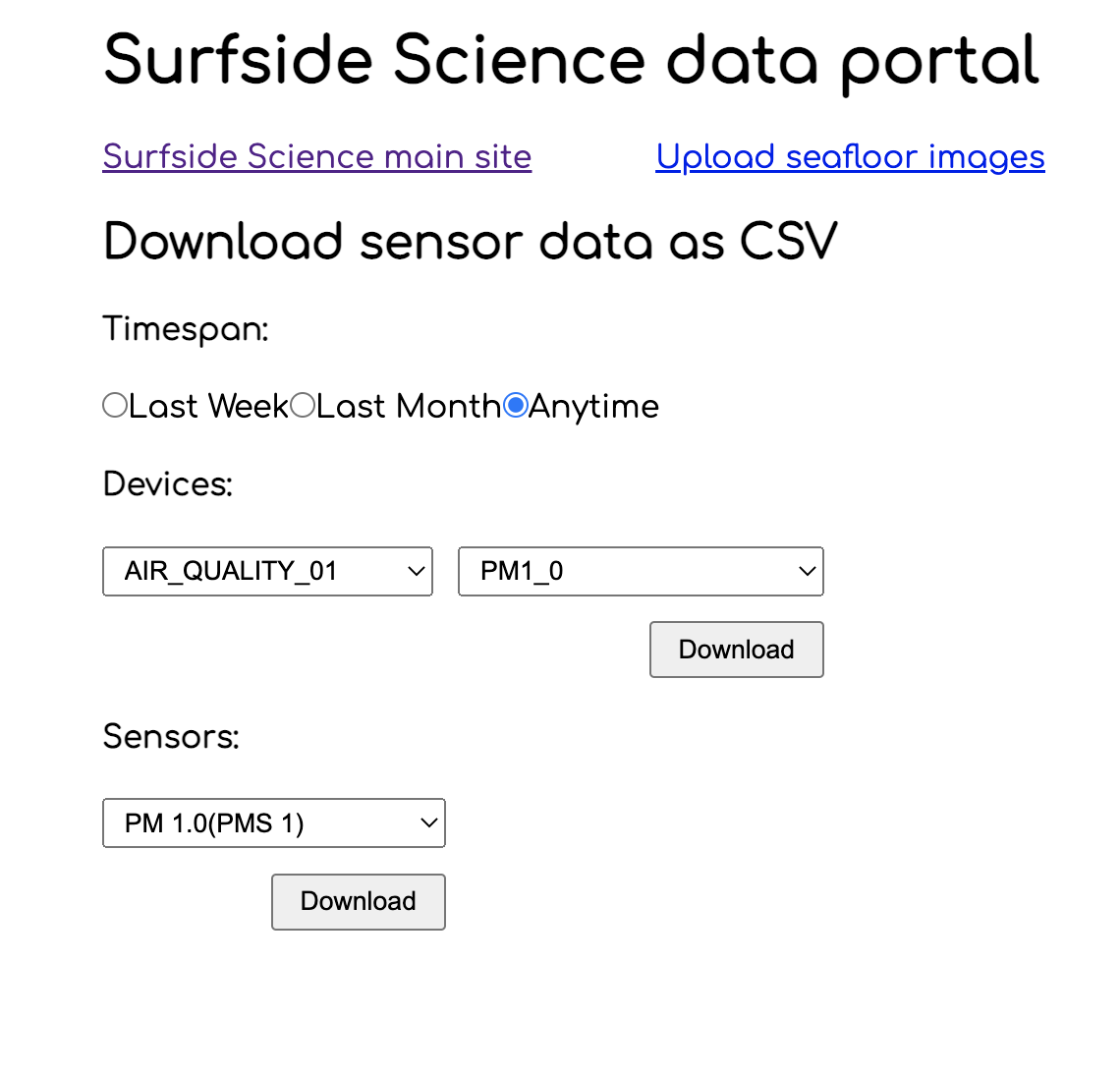
Our environmental science data portal is a simplified access point for the data described above. It allows you to filter and download data by following the steps below.
Timespan
Select from the options Recent, All, or Custom. Recent will select either the most recent month, if you’re looking for maps, or the past 24 hours if you’re looking at electronic sensors. For image-based seafloor classification data this will be the most recent date of image collection. All includes all available data for the selected parameter, and Custom allows you to specify a date range.
Data selection
Choose the topic, parameter, and location you’re interested in accessing data for. For electronic sensors measuring air and water quality there are multiple parameters measured at each station, for seafloor maps there are two options based on satellite imagery and classified field imagery, and for other maps there is only one option. Finally, there is only one location available currently, which is Surfside. This will hopefully be expanded soon by replicating these methods.
Once you’re finished selecting options, a ‘Download CSV’ button or links will appear to download files with the specified data.
Examples
Following below are details for accessing and working with each data type described above, along with examples. Tools used in the process will be mentioned as needed, but installation guides and downloads are linked here for easy reference:
CSV example: Particulate Matter PM_2.5
- Download data
- Go to the data portal website https://data.brenchies.com/
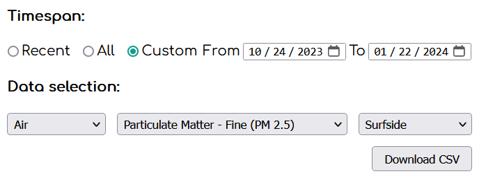
- For Timespan, select Custom to choose a date range
- Adjust From for about 3-4 months ago, and To for today
- For Data selection, select Topic > Parameter > Location as Air > Particulate Matter – Fine (PM 2.5) > Surfside
- Click ‘Download CSV’
- Get an overview
- Open our helper spreadsheet for particulate matter data and click File > Make a copy
- Rename it for yourself
- Switch to the tab for the Raw datasheet at the bottom
- In the menu go to File > Import > Upload > Browse and select the CSV file you just downloaded
- Select the option to ‘Replace current sheet’ and select ‘Comma’ as separator type
- Select the first column of the data in the Raw sheet and ctrl C to copy it
- Switch to the Data tab and select the first column and ctrl V to paste the copied column
- Select the second row in the Data tab for columns B to G and double click the dot in the bottom right to fill down
- Switch to the Summary tab to see your data
GeoTIFF: Mangrove vegetation maps
- Download data
- Go to the data portal website https://data.brenchies.com/
- For Timespan, select All to get a list of all available maps
- For Data selection, select Topic > Parameter > Location as Vegetation > Satellite Maps > Surfside
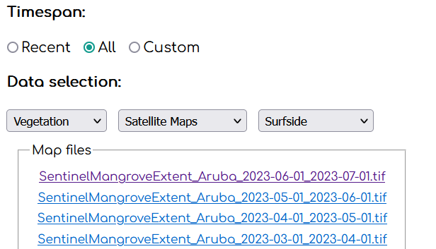
- Click on a file of your choice called SentinelMangroveExtent_Aruba_YYYY-MM-DD-YYYY-MM-DD.tif to download it
- Next scroll down a bit and pick an older map to compare to
- Click on the file to download the map from that date
- Open maps to compare
- Open QGIS on your computer
- Create a new project
- Add the .tif files you just downloaded to the map
- The map has values of 1 for pixels classified as mangroves, and 0 for non-mangroves
- Go to Processing > Toolbox in the menu
- Under Raster analysis, find Raster layers unique values report and double click it to run the tool
- Select the Input layer for the first map, and change the bottom option to ‘Create Temporary Layer’ and click ‘Run’
- Rename the temporary layer with the date and topic of the map you just ran it on
- Repeat for the other map
- Right click on the two tables to get the total count of pixels classified as mangrove
- Multiply these by 100 to get the area of mangroves in square meters for each timepoint
GeoTIFF: Satellite-based seafloor classification
- Download data
- Go to the data portal website https://data.brenchies.com/
- For Timespan, select All to get a list of all available maps
- For Data selection, select Topic > Parameter > Location as Seafloor > Satellite Maps > Surfside
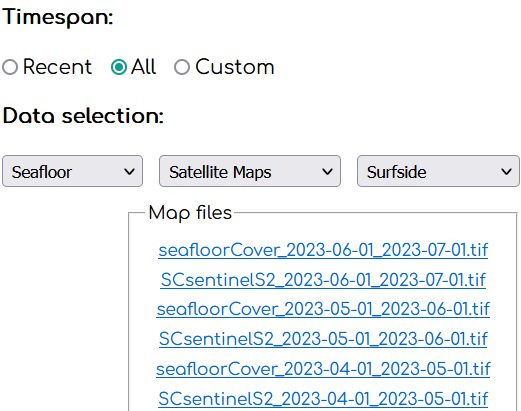
- Click on a file of your choice called seafloorCover_YYYY-MM-DD-YYYY-MM-DD.tif to download it
- If you want to also look at the Sentinel-2 satellite imagery which was used to create the map, you can also download SCsentinelS2_YYYY-MM-DD-YYYY-MM-DD.tif
- Next scroll down a bit and pick an older map to compare to
- Click on the file to download the map from that date
- Open maps to compare
- Open QGIS on your computer
- Create a new project
- Add the .tif files you just downloaded to the map
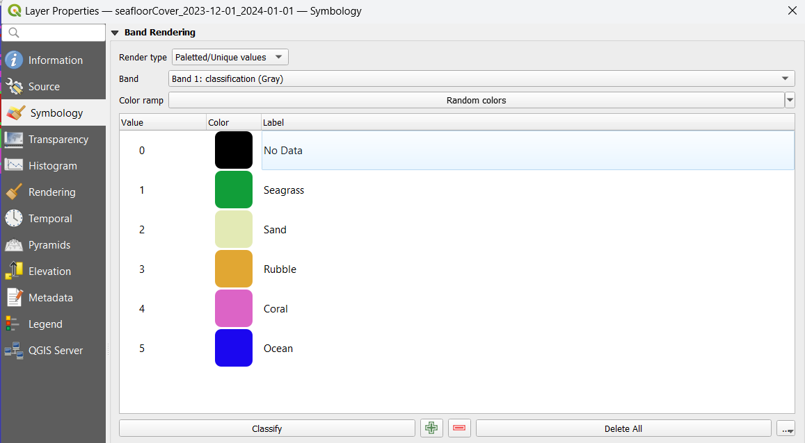
- The classification key is as follows:
- 1 = Seagrass
- 2 = Sand
- 3 = Rubble
- 4 = Coral
- 5 = Ocean
- Double click on one of your maps, go to Symbology, select Render type as Palleted/Unique Values, then click Classify, then adjust your colors and labels to match the classes they represent
- In the bottom right, click the little dots with arrow thing to save the colors and labels
- Click OK to save
- Double click on the other maps, and under Symbology find the little three dots and arrow button and load the saved colors and labels to match your other map
- Go to Processing > Toolbox in the menu
- Under Raster analysis, find Raster layers unique values report and double click it to run the tool
- Select the Input layer for the first map, and change the bottom option to ‘Create Temporary Layer’ and click ‘Run’
- Rename the temporary layer with the date and topic of the map you just ran it on
- Repeat for the other map
- Right click on the two tables to get the total count of pixels classified as each seafloor type
- Multiply these by 100 to get the areas in square meters for each timepoint
- Copy them to a table for comparison
More examples coming soon:
- CSV: Reef islands
- CSV: Image-based seafloor classification
- Shapefile: Coastline
- Shapefile: Reef islands